A music visualizer can show the signal directly, drive a numerical
model, or map musical features to geometry. These notes explain which
choice each view makes, and what its image can tell you.
This is an interactive demonstrator with a technical report. A numerical
reconstruction and modal-refinement comparison is complete; it is not a
peer-reviewed paper. The listener study remains a proposal.
Read the report and results ↗
Five colored grain populations follow the strongest peak in their
own ranges: Sub 20–60 Hz, Bass 60–250 Hz, Mids 250–2,000 Hz, Highs
2,000–6,000 Hz, and Air 6,000–16,000 Hz. They do not isolate
instruments.
Each peak drives the complex harmonic response of a scaled virtual
plate with 36 sine modes. A continuously selected phase displays
interior nodal curves. Transition smoothing defaults to 0.12
seconds; coefficient changes preserve all grain positions. There
is no preset shape catalog or target projection.
Every simply supported sine mode is zero at the rim. This view
divides out their shared boundary factor without changing interior
zeros of the selected phase slice. Faster bounded drift, a soft
inward rim force, and diffusion emphasize readable forms. About
18% of grains remain looser to retain motion and finite-width
clusters.
These are declared display choices, not validated dry-sand
mechanics or the response of the original metal plate. Low bands
use an 8,192-sample FFT; upper bands use 2,048 samples. Frequency
changes therefore have a finite resolution and response time.
Measured layers retains version 0.4's three softly filtered copies
of the sixteen-mode plate. Plate model retains its original
broadband calculation: a 0.30 m square in Fit, or the visible
rectangle with a 0.30 m short edge in Fill, 2 mm thick, E = 200
GPa, density = 7,800 kg/m³, Poisson ratio 0.30, damping 0.015, and
fractional exciter position (0.41, 0.38). Their boundary nodes
remain visible.
A 72 × 72 grid advances a damped wave equation with fixed edges at
a numerical step of 1/180. Two sources share a 1.8 Hz visual
frequency, with a π/3 phase offset. Input RMS controls forcing
strength.
The simulation uses normalized units and a separate visual clock.
Contours are normalized to the current field amplitude. Source
locations and visible frequency are design choices; they do not
reproduce a particular fluid experiment.
03 / Stereo trace
x(t) = L(t) y(t) = R(t)
Pairs of channel samples form a phase portrait. Identical channels
produce a line; generated tones with rational frequency ratios
produce repeating loops.
The tone preview uses analytic sine functions. During playback,
the trace uses synchronized left/right samples from one
2,048-sample AudioWorklet window. File and capture pause retains
that last measured window. Display gain changes the size of the
trace, not the audio.
04 / Spectrum
Δf = sample rate / 4096 T = 4096 / sample rate
A 4,096-sample Web Audio FFT with a Blackman window. At 48 kHz,
the window spans 85.33 ms and bins are spaced 11.72 Hz apart. Bars
show band maxima on a log-frequency axis.
Analyser smoothing is 0.65. The displayed magnitude is relative
and clipped between −100 and −20 dB. It is not calibrated power.
Paused tone previews mark synthetic frequencies. Paused files and
capture retain the last measured spectrum; they do not switch to a
synthetic tone.
05 / Flow orb
v = p × ∇Ψ
q̈ + 2ζωq̇ + ω²q = ω² F(sound,t)
Independent trails retain their curl-driven flow and 80-position
histories. A shared liquid envelope gives bass broad order-2
waves, mids order-3 folds and treble order-4 ripples. Damped
oscillators react to the band envelopes and release toward a
sphere in silence.
The relative oscillation rates use the Rayleigh mode ordering
reviewed by
Easter, Bojarevics and Pericleous (2011). Our forcing, visible time scale, damping and 0.17 deformation
cap are display choices. A sampled volume correction normalizes
the shared envelope at its current base radius; loudness slightly
changes that radius.
The tangent velocity construction is motivated by
Bridson, Hourihan and Nordenstam (2007). Numerical advection, independent radial layers and surface
deformation do not constitute a calibrated fluid simulation. There
is no pressure or viscosity solver.
06 / Constellation
relative cell magnitude → spring target
recent maximum →
              fading peak tip
Fixed rays follow 64 logarithmic display cells from 40 to 16,000
Hz. Each ray extends with its cell's relative strength, gated by
overall loudness. A damped 3 Hz visual spring smooths extension
and return. A faint outer tip holds the recent maximum with a
0.45-second exponential decay.
Directions and assignments stay fixed, making the changes
traceable to sound. The default has 129 rays. Color labels broad
frequency ranges; low cells can share an FFT bin. This is a
spectral display with chosen dynamics, not source separation or a
stellar model.
TECHNICAL REPORT / REPRODUCIBLE PLATE COMPARISON
Interference, and the limits of sixteen modes.
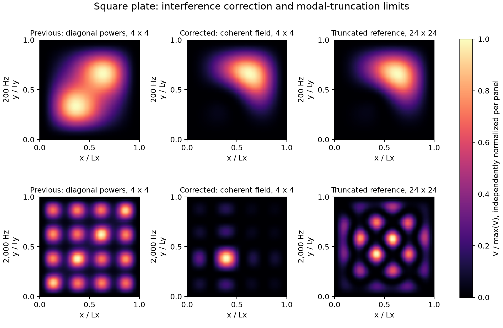
Plate model and Measured layers use the full second-moment field:
V(x,y) = sum_i sum_j B_i(x,y) B_j(x,y) mean(q_i q_j). A common
sinusoid drives different natural-frequency groups at the same forcing
frequency. Their cross terms therefore matter. This is the
reconstruction tested in the report, before particle motion or display
normalization.
The saved comparison uses a unit sinusoidal point force, an 81 × 81
grid, five drive frequencies and aspect ratios 1 and 1.5. Same-bank
agreement checks the formula for the retained modes. A separate 4 × 4
versus 24 × 24 modal comparison checks truncation; the larger
reference is still an approximation. Tiny reconstruction errors do not
imply accurate real sand or a complete high-frequency plate model.
These links select Tone, the fitted square Plate model and an optional
grayscale activity overlay. All normal views and controls remain
available. Dark areas are quiet, light areas active; the field is
normalized to its own maximum. Grains remain visible and are governed
by illustrative transport. Play tone switches from analytical preview
to measured worklet second moments.
Loading the saved numerical results…
Relative spatial L2 errors before display normalization
Aspect
Drive, Hz
Previous diagonal, %
Coherent same-bank, fraction
4 × 4 vs 24 × 24, %
Each panel is independently normalized to show geometry. The
numerical errors above use raw fields. These are calculated activity
fields, not photographs or measured grain distributions.
A separate 2,048-sample analyser supplies faster music features; at 48
kHz its window spans 42.67 ms. The 3D features use a 0.025-second
attack and 0.13-second release envelope. Spectrum keeps its longer
4,096-sample window. These window sizes are not measurements of total
visual latency.
Frequency colors keep each population's color fixed: five in Five-band
sand and three in the other views. Grain identities are interleaved
throughout the plate; orb strands and constellation directions retain
their seeded bands. Five-band sand follows spectral peaks, while
Measured layers uses three softly filtered input banks. Spectrum
assigns colors by frequency; wave colors follow contour levels. These
mappings do not isolate voices or instruments.
Sound palette shifts the selected palette smoothly when positive
spectral change crosses an adaptive threshold. Colors coexist instead
of flashing the whole view between flat colors. The cue follows the
positive spectral-change principle described in
librosa’s onset-strength documentation, with a custom linear-magnitude calculation and gate. It is not a
benchmarked onset detector or beat tracker. Single color remains
available for monochrome or a chosen tint.
Sand starts with 15,000 grains: 3,000 in each of its five frequency
populations, or 5,000 in each measured layer. Settings can increase
the total to 90,000. Adding grains preserves existing positions. Fill
canvas uses a complete rectangular plate and wave domain. Grain size
stays fixed, and every boundary remains visible. Rectangular
dimensions change modal frequencies and spatial derivatives. Toggle it
off to return to the square. The 3D views keep their full proportions.
A QUICK WALKTHROUGH / RECORDED TEST NOTES
Sound, given shape.
Choose Demo music to hear a locally generated sixteen-second passage.
Switch between Flow orb and Constellation: the bass, chord, arpeggio,
and percussion sections drive the same measured audio pipeline as an
uploaded track. Pause holds the current shape; Tone supplies a steady
signal for comparison.
To inspect physical resonance, choose Sand → Appearance → Plate model,
then open Adjust beside the Tone label and try the 267 Hz preset. Move
the slider a little, then return to the preset. The frequency you hear
drives the plate; the listening-volume slider only changes what
reaches the speakers.
The sand reference began with three photographs, labeled 345, 3835,
and 3975 Hz. Copying those numbers into a program would not reproduce
the pictures. The plate's dimensions, thickness, supports, and point
of excitation all affect its resonances. The photographs show a center
fastening. Our square has supported edges.
That choice gives us sine modes we can calculate directly. Plate model
retains sixteen modes; Five-band sand uses thirty-six on each scaled
virtual plate. Plate model and Measured layers retain the full modal
second-moment matrix, including interference between groups. Their
sixteen-mode bank remains a low-order approximation: the numerical
comparison found substantial high-frequency truncation errors,
especially in rectangular plates. Five-band sand is a separate
designed musical mapping.
The grains are a second model. Plate model retains normalized
position-dependent diffusion. Measured layers adds a low-activity
attraction baseline, overlapping band input, and slower relative field
envelopes. Both keep stochastic motion and reflecting boundaries.
These rendering choices have not been experimentally calibrated, so
they cannot estimate settling time in a real experiment. Five-band
sand additionally chooses a phase slice, removes the shared boundary
factor, and uses faster bounded drift with a soft rim force. These
choices emphasize interior patterns while preserving continuous grain
positions.
For a simpler picture of the signal, switch to Stereo trace. Left goes
horizontally, right vertically. Identical channels give you a line.
The 3:2 generated-tone option gives you a loop. A music file can look
quite different.
Wave field uses two slow sources, driven in strength by the audio. Its
ripples have their own clock. Spectrum uses a 4,096-sample FFT:
roughly 85 ms per window at 48 kHz. The bars report relative
magnitude.
One useful check is already reproducible: at the modeled 535 Hz
resonance, the browser's modal mean-square response was 0.9933 times
the analytic prediction in the recorded test. That's a check of the
oscillator pipeline, not experimental validation of the grains.
Open a local audio file when you're ready. It stays on your device.
You can also open a YouTube link, play the video, and use Connect tab
audio. Select the playing browser tab and enable Share audio. The
embedded player supplies playback; the browser supplies the audio
stream after your permission. Captured audio is analyzed without being
replayed. Pause visuals stops analysis while the video can continue
playing.
AI-ASSISTED PROJECT
Development notes.
Developed with the help of AI tools, including Codex. AI assistance
was used in literature exploration, technical writing, implementation,
and numerical verification. The technical report documents the
methods, reproducible results, and model limitations.
The wider review considers fifteen visualization families, including
reaction–diffusion, fluid flow, coupled oscillators, swarmalators, and
spectral geometry. The bibliography contains 63 references and records
whether each paper was inspected in full or through its abstract and
metadata.
One proposed study compares physical, direct musical, and hybrid
control within the same plate scene. Another compares stochastic
particles with a continuum density solver. Both require controlled
inputs, defined error measures, and reproducible experiments.
A public repository, demonstration, and archived report can make the
work inspectable. A scholarly claim needs an original contribution and
supporting results. Neither an archive DOI nor a polished website
establishes peer review.